Implementing and Visualizing SVM in Python with CVXOPT

So this post is not about some great technical material on any of the mentioned topics. I have been trying to use cvxopt to implement an SVM-type max-margin classifier for an unrelated problem on Reinforcement Learning. While doing that, I had trouble figuring out how to use the cvxopt library to correctly implement a quadratic programming solver for SVM. Since I eventually figured it out, I am just sharing that here. Let us get into it then.

Generating the data

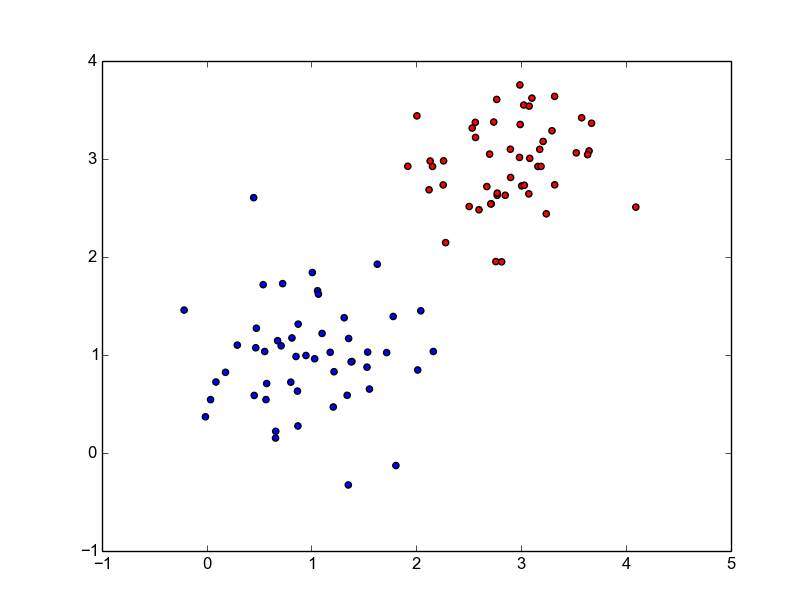
We will generate linearly separable, 2-class data using 2-dimensional Gaussians. Below is the entire Python code to generate, visualize and save the data.

import pickle
import numpy as np
import matplotlib.pyplot as plt

DIM = 2
COLORS = ['red', 'blue']

# 2-D mean of ones
M1 = np.ones((DIM,))
# 2-D mean of threes
M2 = 3 * np.ones((DIM,))
# 2-D covariance of 0.3
C1 = np.diag(0.3 * np.ones((DIM,)))
# 2-D covariance of 0.2
C2 = np.diag(0.2 * np.ones((DIM,)))

def generate_gaussian(m, c, num):
    return np.random.multivariate_normal(m, c, num)

def plot_data_with_labels(x, y):
    unique = np.unique(y)
    for li in range(len(unique)):
        x_sub = x[y == unique[li]]
        plt.scatter(x_sub[:, 0], x_sub[:, 1], c = COLORS[li])
    plt.show()

NUM = 50
if __name__ == '__main__':
    # generate 50 points from gaussian 1
    x1 = generate_gaussian(M1, C1, NUM)
    # labels
    y1 = np.ones((x1.shape[0],))
    # generate 50 points from gaussian 2
    x2 = generate_gaussian(M2, C2, NUM)
    y2 = -np.ones((x2.shape[0],))
    # join
    x = np.concatenate((x1, x2), axis = 0)
    y = np.concatenate((y1, y2), axis = 0)
    print('x {} y {}'.format(x.shape, y.shape))
    plot_data_with_labels(x, y)
    # write
    with open('gaussiandata.pickle', 'wb') as f:
        pickle.dump((x, y), f)

The code has comments and should be an easy read. It will generate a pickle file with the generated data and a plot that looks like below.

Fitting an SVM

Now for the second part, let us look at the SVM formulation and the interface that CVXOPT provides. Below is the primal SVM objective.

$$\begin{eqnarray} \min_{w}\frac{1}{2}||w||^{2} \nonumber \\\ \textrm{s.t.}\quad y_{i}(w^{T}x_{i} + b) \ge 1 \quad \forall i \end{eqnarray}$$

And this is the corresponding dual problem.

$$\begin{eqnarray} \min_{\alpha}\frac{1}{2} \alpha^{T}K\alpha - 1^{T}\alpha \nonumber \\\ \textrm{s.t.}\quad \alpha_{i} \ge 0 \quad \forall i \\\ \textrm{and}\quad y^{T}\alpha = 0 \end{eqnarray}$$

This is all good. Now below is the interface that cvxopt provides. They have a QP solver and it can be called as cvxopt.solvers.qp(P, q[, G, h[, A, b[, solver[, initvals]]]]). The problem that this solves is-

$$\begin{eqnarray} \min_{x}\frac{1}{2} x^{T}Px - q^{T}x \nonumber \\\ \textrm{s.t.}\quad Gx \preceq h \\\ \textrm{and}\quad Ax = b \end{eqnarray}$$

All we need to do is to map our formulation to the cvxopt interface. We are already almost there. \(\alpha\)s are the \(x\)s, \(K\) is the \(P\), \(q\) is a vector of ones, \(G\) will be an identity matrix with \(-1\)s as its diagonal so that our greater than is transformed into less than, \(h\) is vector of zeros, \(A\) is \(y^{T}\) and \(b\) is 0. That is all we need to do. So below is the code that does that given the training data x and labels y.

def fit(x, y): 
    NUM = x.shape[0]
    DIM = x.shape[1]
    # we'll solve the dual
    # obtain the kernel
    K = y[:, None] * x
    K = np.dot(K, K.T)
    P = matrix(K)
    q = matrix(-np.ones((NUM, 1)))
    G = matrix(-np.eye(NUM))
    h = matrix(np.zeros(NUM))
    A = matrix(y.reshape(1, -1))
    b = matrix(np.zeros(1))
    solvers.options['show_progress'] = False
    sol = solvers.qp(P, q, G, h, A, b)
    alphas = np.array(sol['x'])
    return alphas

Note that sol['x'] contains the \(x\) that was part of cvxopt interface - it is our \(\alpha\). Now if you are familiar with SVMs, you will know that only a few of the alphas should be non-zero and they will be our support vectors. Using these alphas, we can obtain \(w\) and \(b\) from our original SVM problem. Once we do that, they will together define the decision boundary. \(w\) is equal to \(\Sigma_{i}\alpha_{i}y_{i}x_{i}\) and \(b\) is equal to \(y_{i} - w^{T}x_{i}\) for any \(i\) such that \(\alpha_{i} \gt 0\). So we do the following to obtain them.

# fit svm classifier
alphas = fit(x, y)

# get weights
w = np.sum(alphas * y[:, None] * x, axis = 0)
# get bias
cond = (alphas > 1e-4).reshape(-1)
b = y[cond] - np.dot(x[cond], w)
bias = b[0]

Finally, we’ll plot the decision boundary for good visualizaiton. Since it will be a line in this case, we need to obtain the slope and intercept of the line from the weights and bias. Here is the code.

def plot_separator(ax, w, b): 
    slope = -w[0] / w[1]
    intercept = -b / w[1]
    x = np.arange(0, 6)
    ax.plot(x, x * slope + intercept, 'k-')

The entire code is on my github. Once we run it, we get the following final plot.

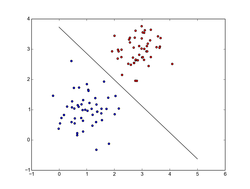
Looks pretty neat and is good for visualizing 2-D stuff.

References: