Building autoencoders in Lasagne
04 Jun 2016 ▪ 0 CommentsAutoencoders are generally used in unsupervised data learning settings. When we have unlabeled data, we can use an autoencoder to learn an internal, low-dimensional representation of the input data. The model does not need output labels, rather the output is supposed to be the reconstruction of the input data itself. The errors are propagated back and slowly we can expect the model to learn a well encoded representation of the input data.
A simple autoencoder
Let's build a simple model with an input layer, a hidden (encoded) layer and an output layer.
First, let's get done with the imports and define model parameters.
import matplotlib.pyplot as plt
import pylab
import pickle
import numpy as np
import theano
import lasagne

MODEL_FILE = 'mnist.state_ae.model.lasagne'    # File to store the learned model

N_ENCODED = 32    # Size of encoded representation
NUM_EPOCHS = 50   # Number of epochs to train the net
BATCH_SIZE = 200  # Batch Size
NUM_FEATURES = 28 * 28 # Input feature size
Next, define a function to generate batches of data.
def gen_data(data, p, batch_size = BATCH_SIZE):

    x = np.zeros((batch_size,NUM_FEATURES))
    for n in range(batch_size):
        x[n,:] = data[p+n, :]

    return x, x
Build the network:
def build_network():
    print("Building network ...")

    # Define the layers
    l_in = lasagne.layers.InputLayer(shape=(None, NUM_FEATURES))
    encoder_l_out = lasagne.layers.DenseLayer(l_in,
                                    num_units=N_ENCODED,
                                    W = lasagne.init.Normal(),
                                    nonlinearity=lasagne.nonlinearities.rectify)
    decoder_l_out = lasagne.layers.DenseLayer(encoder_l_out,
                                    num_units = NUM_FEATURES,
                                    W = lasagne.init.Normal(),
                                    nonlinearity = lasagne.nonlinearities.sigmoid)

    # Define some Theano variables
    target_values = theano.tensor.fmatrix('target_output')
    encoded_output = lasagne.layers.get_output(encoder_l_out)
    network_output = lasagne.layers.get_output(decoder_l_out)

    cost = lasagne.objectives.squared_error(network_output,target_values).mean()
    all_params = lasagne.layers.get_all_params(decoder_l_out,trainable=True)

    # Compute AdaDelta updates for training
    updates = lasagne.updates.adadelta(cost, all_params)

    # Some Theano functions
    train = theano.function([l_in.input_var, target_values],
                            cost,
                            updates=updates,
                            allow_input_downcast=True)
    predict = theano.function([l_in.input_var],
                                network_output,
                                allow_input_downcast=True)
    encode = theano.function([l_in.input_var],
                                encoded_output,
                                allow_input_downcast=True)

    return train, predict, encode
Now, we will use the above model. I have the MNIST dataset dumped in a file using pickle.
The data is normalized to be between 0 and 1, and reshaped to be of shape (784, ) from the original (1, 28, 28).
After loading the dataset into train and test variables, we proceed to train the model.
import state_ae

def main():
    # Load the dataset
    print("Loading data...")

    f = open('x_train.mnist', 'rb')
    x_train = pickle.load(f)
    f.close()
    f = open('x_test.mnist', 'rb')
    x_test = pickle.load(f)
    f.close()

    trainfunc, predict, encode = state_ae.build_network()
    learn(x_train, trainfunc, x_test)
    check_model(x_test, predict, encode)

def learn(x_train, trainfunc, x_test):

    for it in range(state_ae.NUM_EPOCHS):

        p = 0
        count = 0
        avg_cost = 0
        while True:
            x, y = state_ae.gen_data(x_train, p)
            p += len(x)
            count += 1
            avg_cost += trainfunc(x, y)

            if (p == len(x_train)):
                break

        print("Epoch {} average loss = {}".format(it, avg_cost / count))
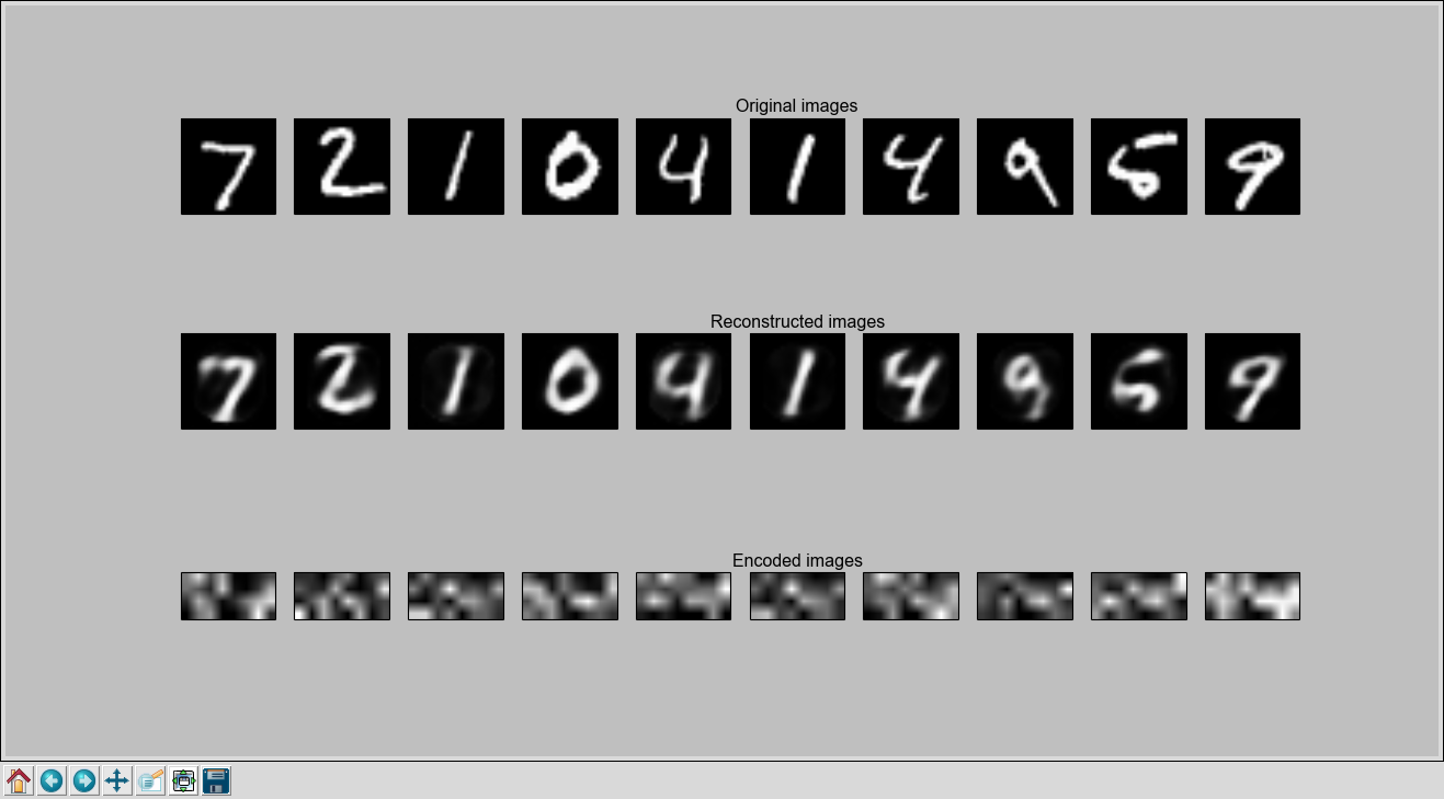
We train the network for 50 epochs. After that it seems to reach a reasonably good error of 0.023. Now we will plot the images and visualize the results.
def check_model(x_test, predict, encode):

    encoded_imgs = encode(x_test[:, :])
    decoded_imgs = predict(x_test[:, :])

    import matplotlib.pyplot as plt

    n = 10  # how many digits we will display
    plt.figure(figsize=(40, 8))
    for i in range(n):
        # display original
        ax = plt.subplot(3, n, i + 1)
        plt.imshow(x_test[i].reshape(28, 28))
        plt.gray()
        ax.get_xaxis().set_visible(False)
        ax.get_yaxis().set_visible(False)
        if (i == n / 2):
            ax.set_title("Original images")

        # display reconstruction
        ax = plt.subplot(3, n, i + n + 1)
        plt.imshow(decoded_imgs[i].reshape(28, 28))
        plt.gray()
        ax.get_xaxis().set_visible(False)
        ax.get_yaxis().set_visible(False)
        if (i == n / 2):
            ax.set_title("Reconstructed images")

        # display encodings
        ax = plt.subplot(3, n, i + 2*n + 1)
        plt.imshow(encoded_imgs[i].reshape(4, 8))
        plt.gray()
        ax.get_xaxis().set_visible(False)
        ax.get_yaxis().set_visible(False)
        if (i == n / 2):
            ax.set_title("Encoded images")

    plt.show()
This is what we get.

The autoencoder does a rather good job at learning encodings and reconstructing the digits from them. The last row shows the 32 dimensional encoding learned for each of the ten test images (in a 4x8 sized image).
Find the entire working code for this autoencoder in Lasagne on my github.