Learning to predict a mathematical function using LSTM

In my previous post, I shared how I used Python to generate sequential and periodic data from a sine wave. I dumped this data into a file called sinedata.md last time, and we are going to use that dump in this post.

For the LSTM, I have used the library called Lasagne. It is a great library for easily setting up deep learning models. Also, they provide some "Recipes" for quick setup. I have used the LSTM model they provided for text generation and modified it to suit my needs for learning a sine-wave. So I will only share the relevant code in this post to avoid the clutter.

First we'll use pickle to load the data that was generated earlier:

in_file = open('sinedata.md', 'rb')
in_text = pickle.load(in_file)

The parameters used for the LSTM are as below:

# Sequence Length
SEQ_LENGTH = 50

# Number of units in the two hidden (LSTM) layers
N_HIDDEN = 32

# Optimization learning rate
LEARNING_RATE = .01

# All gradients above this will be clipped
GRAD_CLIP = 100

# How often should we check the output?
PRINT_FREQ = 10

# Number of epochs to train the net
NUM_EPOCHS = 50

# Batch Size
BATCH_SIZE = 64

The LSTM architecture contains just 1 hidden layer with a tanh non-linearity. The output layer has linear non-linearity. There is only 1 output unit. So given the last 50 sine wave samples at a distance of 0.1 x-units each, our network will learn to predict the 51st point. Then given the last 49 samples from the data and the generated sample as the 50th sample, our network will predict the 51st sample once again. It will keep doing this, moving forward in time, for ~200 time steps in our case.

So, for this experiment, I have generated sine-wave data for x ranging from 0 to 2000 at a gap of 0.1. I train the LSTM on this data.

The gif below shows what the network predicted after each training iteration.

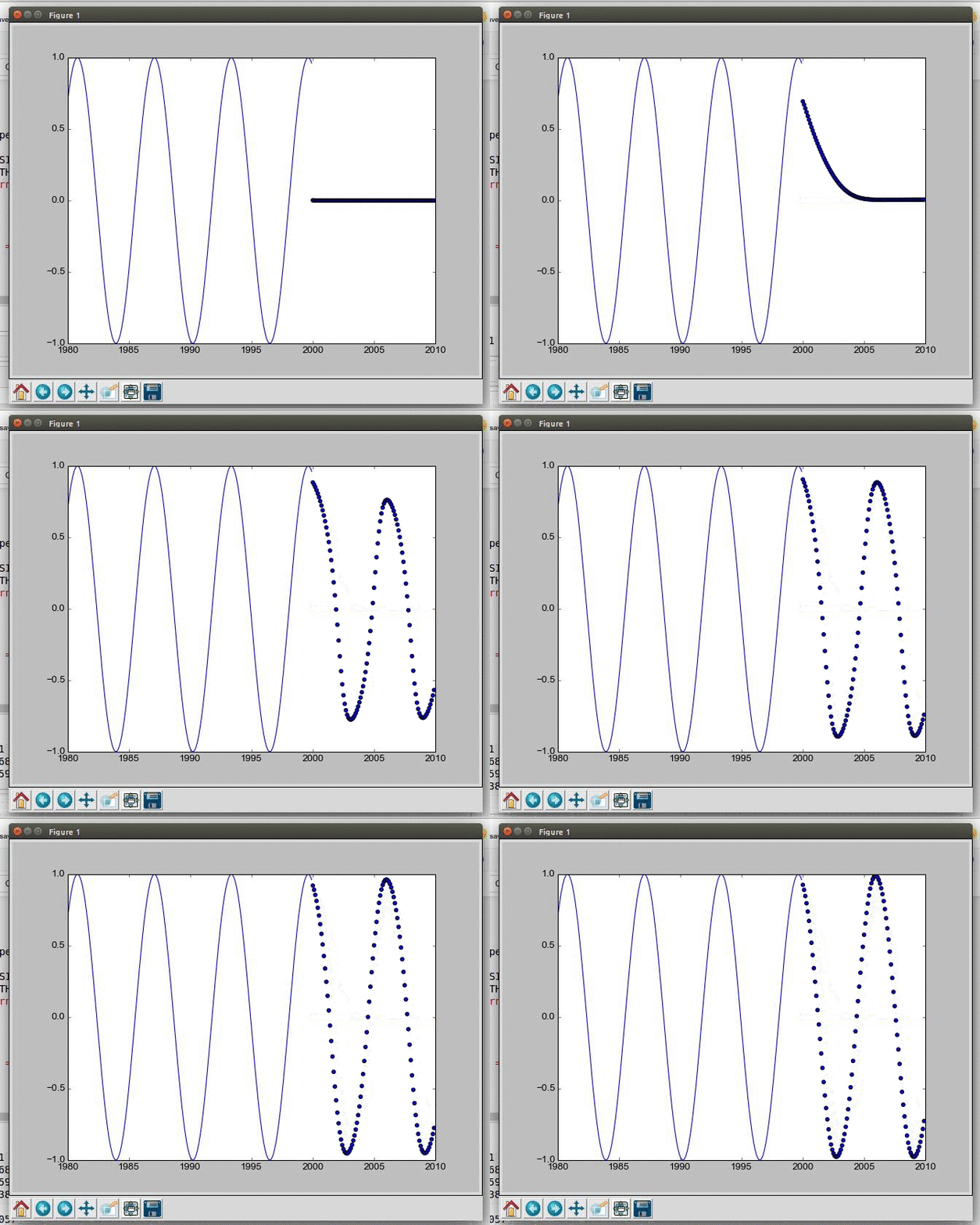
Some things to note:

• The network does not take much time to train; probably because of the sequence length of 50 and 32 hidden units
• The prediction is almost perfect
• The network can be trained using continuous data and also to predict continuous data

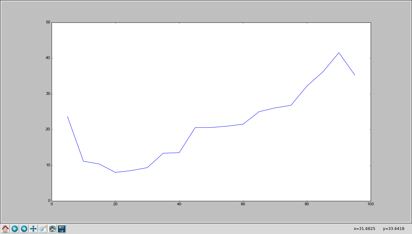
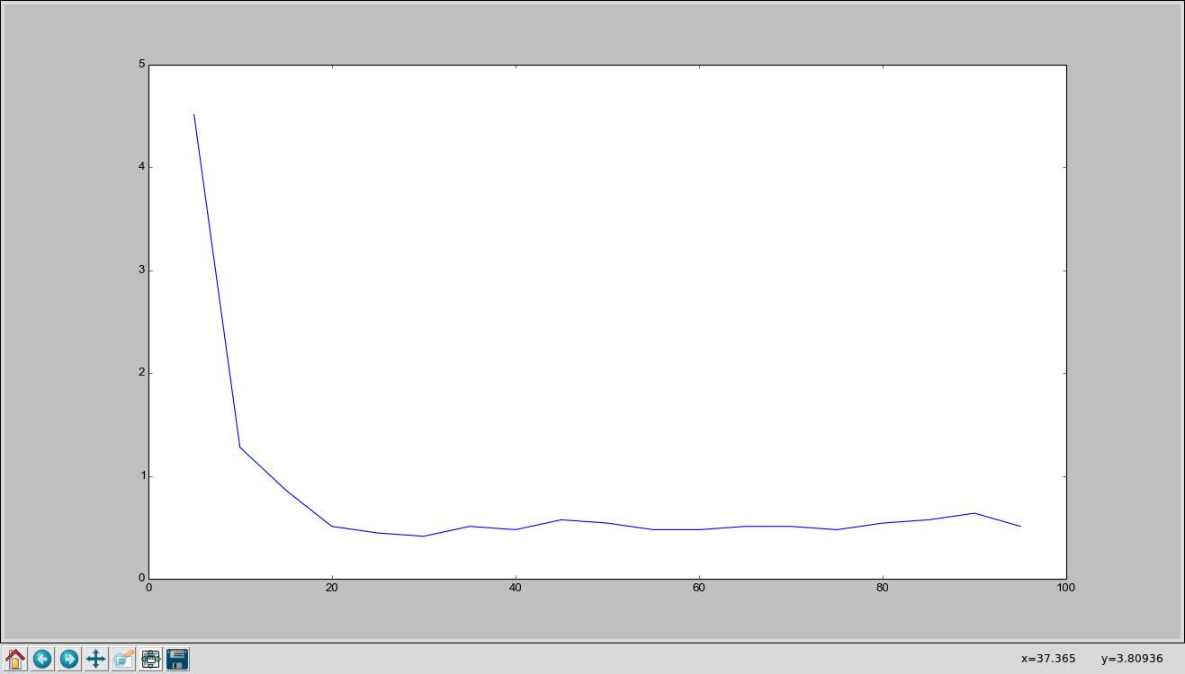
Let us track the variation of training time and number of required epochs with change in sequence length. The target training error is < 0.0001.

Time Taken vs Sequence Length

Number of Epochs vs Sequence Length

Some things to note:

• Sequence length of 20 seems to be enough for training error of the order of 0.0001
• Time taken increases as sequence length goes beyond 20, which is expected because of the increased complexity of the model
• Number of epochs remains the same more or less, for sequence length beyond 20

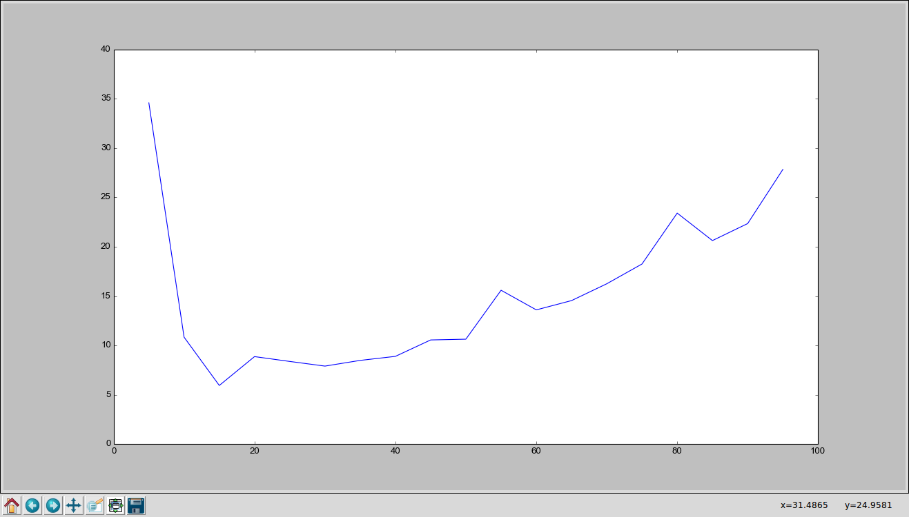
Let us now track the variation of training time and number of required epochs with change in the number of units in the hidden layer of the LSTM. The target training error is again < 0.0001.

Time Taken vs # Hidden Units

Number of Epochs vs # Hidden Units

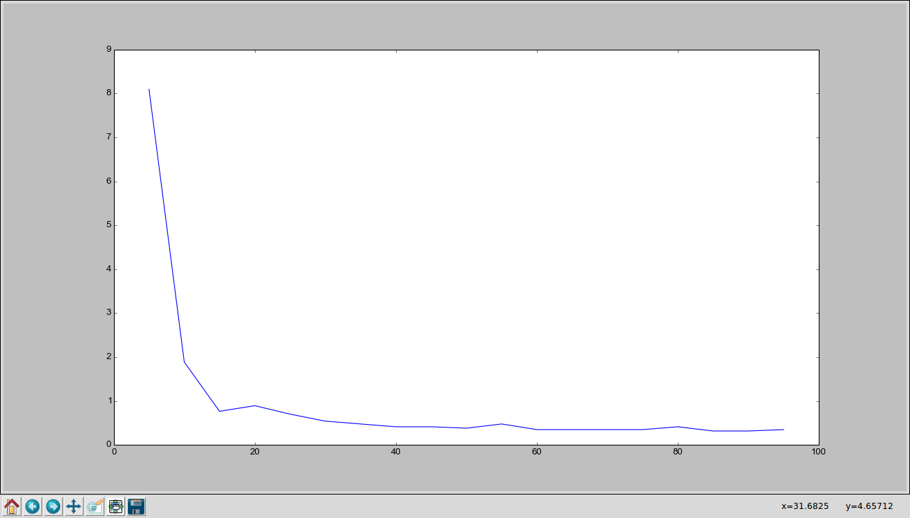
Some things to note:

• ~15 seems to be a reasonable number of hidden units for training error of the order of 0.0001
• Time taken increases as number of hidden untis goes beyond 15, which is expected because of the increased complexity of the model
• Number of epochs remains the same more or less

A possible explanation for these observations is that the sine-wave is pretty easy to learn. If the network knows the last ~20 values, it can predict what the next value should be. This optimal sequence length should be higher for more complex functions. Also the number of hidden units of ~15, seems to be good for learning to model a sine-wave.