Implementing Fisher’s LDA from scratch in Python
04 Oct 2016 ▪ 0 CommentsWhat?
As mentioned above, Fisher’s LDA is a dimension reduction technique. Such techniques can primarily be used to reduce the dimensionality for high-dimensional data. People do this for multiple reasons - dimension reduction as feature extraction, dimension reduction for classification or for data visualizaiton.
How?
Since this is the theory section, key takeaways from it are as follows (in case, you do not want to spend time on it)
1. Calculate \(S_{b}\), \(S_{w}\) and \(d^{\prime}\) largest eigenvalues of \(S_{w}^{-1}S_{b}\).
2. Can project to a maximum of \(K - 1\) dimensions.
The core idea is to learn a set of parameters \(w \in \mathbb{R}^{d \times d^{\prime}}\), that are used to project the given data \(x \in \mathbb{R}^{d}\) to a smaller dimension \(d^{\prime}\). The figure below (Bishop, 2006) shows an illustration. The original data is in 2 dimensions, \(d = 2\) and we want to project it to 1 dimension, \(d = 1\).
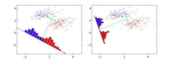
If we project the 2-D data points onto a line (1-D), out of all such lines, our goal is to find the one which maximizes the distance between the means of the 2 classes, after projection. If we could do that, we could achieve a good separation between the classes in 1-D. This is illustrated in the figure on the left and can be captured in the idea of maximizing the "between class covariance". However, as we can see that this causes a lot of overlap between the projected classes. We want to minimize this overlap as well. To handle this, Fisher’s LDA tries to minimize the "within-class covariance" of each class. Minimizing this covariance leads us to the projection in the figure on the right hand side, which has minimal overlap. Formalizing this, we can represent the objective as follows.
$$J(w) = \frac{w^{\mathsf{T}}S_{b}w}{w^{\mathsf{T}}S_{w}w}$$
where \(S_{b} \in \mathbb{R}^{d \times d}\) and \(S_{w} \in \mathbb{R}^{d \times d}\) are the between-class and within-class covariance matrices, respectively. They are calculated as
$$S_{b} = \sum_{k = 1}^K (m_{k} - m)N_{k}(m_{k} - m)^{\mathsf{T}}$$
$$S_{w} = \sum_{k = 1}^K \sum_{n = 1}^{N_{k}} (X_{nk} - m_{k})(X_{nk} - m_{k})^{\mathsf{T}}$$
where \(X_{nk}\) is the \(n\)th data example in the \(k\)th class, \(N_{k}\) is the number of examples in class \(k\), \(m\) is the overall mean of the entire data and \(m_{k}\) is the mean of the \(k\)th class. Now using Lagrangian dual and the KKT conditions, the problem of maximizing \(J\) can be transformed into the solution
$$S_{w}^{-1}S_{b}w = \lambda w$$
which is an eigenvalue problem for the matrix \(S_{w}^{-1}S_{b}\). Thus our final solution for \(w\) will be the eigenvectors of the above equation, corresponding to the largest eigenvalues. For reduction to \(d^{\prime}\) dimensions, we take the \(d^{\prime}\) largest eigenvalues as they will contain the most information. Also, note that if we have \(K\) classes, the maximum value of \(d^{\prime}\) can be \(K - 1\). That is, we cannot project \(K\) class data to a dimension greater than \(K - 1\). (Of course, \(d^{\prime}\) cannot be greater than the original data dimension \(d\)). This is because of the following reason. Note that the between-class scatter matrix, \(S_{b}\) was a sum of \(K\) matrices, each of which is of rank 1, being an outer product of two vectors. Also, because the overall mean and the individual class means are related, only (\(K - 1\)) of these \(K\) matrices are independent. Thus \(S_{b}\) has a maximum rank of \(K - 1\) and hence there are only \(K - 1\) non-zero eigenvalues. Thus we are unable to project the data to more than \(K - 1\) dimensions.
Code
The main part of the code is shown below. If you are looking for the entire code with data preprocessing, train-test split etc., find it here.
def fit(self):
    # Function estimates the LDA parameters
    def estimate_params(data):
        # group data by label column
        grouped = data.groupby(self.data.ix[:,self.labelcol])

        # calculate means for each class
        means = {}
        for c in self.classes:
            means[c] = np.array(self.drop_col(self.classwise[c], self.labelcol).mean(axis = 0))

        # calculate the overall mean of all the data
        overall_mean = np.array(self.drop_col(data, self.labelcol).mean(axis = 0))

        # calculate between class covariance matrix
        # S_B = \sigma{N_i (m_i - m) (m_i - m).T}
        S_B = np.zeros((data.shape[1] - 1, data.shape[1] - 1))
        for c in means.keys():
            S_B += np.multiply(len(self.classwise[c]),
                               np.outer((means[c] - overall_mean),
                                        (means[c] - overall_mean)))

        # calculate within class covariance matrix
        # S_W = \sigma{S_i}
        # S_i = \sigma{(x - m_i) (x - m_i).T}
        S_W = np.zeros(S_B.shape)
        for c in self.classes:
            tmp = np.subtract(self.drop_col(self.classwise[c], self.labelcol).T, np.expand_dims(means[c], axis=1))
            S_W = np.add(np.dot(tmp, tmp.T), S_W)

        # objective : find eigenvalue, eigenvector pairs for inv(S_W).S_B
        mat = np.dot(np.linalg.pinv(S_W), S_B)
        eigvals, eigvecs = np.linalg.eig(mat)
        eiglist = [(eigvals[i], eigvecs[:, i]) for i in range(len(eigvals))]

        # sort the eigvals in decreasing order
        eiglist = sorted(eiglist, key = lambda x : x[0], reverse = True)

        # take the first num_dims eigvectors
        w = np.array([eiglist[i][1] for i in range(self.num_dims)])

        self.w = w
        self.means = means
        return

    # estimate the LDA parameters
    estimate_params(traindata)
The code is pretty self-explanatory if you followed the theory above and read the comments in the code. Once we estimate the parameters, there are two ways to classify it.
-
Thresholding
In one-dimensional projections, we find a threshold \(w_{0}\), which can be basically the mean of the projected means in the case of 2-class classification. Points above this threshold go into one class, while the ones below go in to the other class. Here is the code to do that.''' Function to calculate the classification threshold. Projects the means of the classes and takes their mean as the threshold. Also specifies whether values greater than the threshold fall into class 1 or class 2. ''' def calculate_threshold(self): # project the means and take their mean tot = 0 for c in self.means.keys(): tot += np.dot(self.w, self.means[c]) self.w0 = 0.5 * tot # for 2 classes case; mark if class 1 is >= w0 or < w0 c1 = self.means.keys()[0] c2 = self.means.keys()[1] mu1 = np.dot(self.w, self.means[c1]) if (mu1 >= self.w0): self.c1 = 'ge' else: self.c1 = 'l' ''' Function to calculate the scores in thresholding method. Assigns predictions based on the calculated threshold. ''' def calculate_score(self, data): inputs = self.drop_col(data, self.labelcol) # project the inputs proj = np.dot(self.w, inputs.T).T # assign the predicted class c1 = self.means.keys()[0] c2 = self.means.keys()[1] if (self.c1 == 'ge'): proj = [c1 if proj[i] >= self.w0 else c2 for i in range(len(proj))] else: proj = [c1 if proj[i] < self.w0 else c2 for i in range(len(proj))] # calculate the number of errors made errors = (proj != data.ix[:, self.labelcol]) return sum(errors) -
Gaussian Modeling
In this method, we project the data points into the \(d^{\prime}\) dimension, and then model a multi-variate Gaussian distribution for each class’ likelihood distribution \(P(x | C_{k})\). This is done by calculating the means and covariances of the data point projections. The priors \(P(C_{k})\) are estimated as well using the given data by calculating \(\frac{N_{k}}{N}\) for each class \(k\). Using these, we can calculate the posterior \(P(C_{k}|x)\) and then the data points can be classified to the class with the highest probability value. These ideas are solidified in the code below.''' Function to estimate gaussian models for each class. Estimates priors, means and covariances for each class. ''' def gaussian_modeling(self): self.priors = {} self.gaussian_means = {} self.gaussian_cov = {} for c in self.means.keys(): inputs = self.drop_col(self.classwise[c], self.labelcol) proj = np.dot(self.w, inputs.T).T self.priors[c] = inputs.shape[0] / float(self.data.shape[0]) self.gaussian_means[c] = np.mean(proj, axis = 0) self.gaussian_cov[c] = np.cov(proj, rowvar=False) ''' Utility function to return the probability density for a gaussian, given an input point, gaussian mean and covariance. ''' def pdf(self, point, mean, cov): cons = 1./((2*np.pi)**(len(point)/2.)*np.linalg.det(cov)**(-0.5)) return cons*np.exp(-np.dot(np.dot((point-mean),np.linalg.inv(cov)),(point-mean).T)/2.) ''' Function to calculate error rates based on gaussian modeling. ''' def calculate_score_gaussian(self, data): classes = sorted(list(self.means.keys())) inputs = self.drop_col(data, self.labelcol) # project the inputs proj = np.dot(self.w, inputs.T).T # calculate the likelihoods for each class based on the gaussian models likelihoods = np.array([[self.priors[c] * self.pdf([x[ind] for ind in range(len(x))], self.gaussian_means[c], self.gaussian_cov[c]) for c in classes] for x in proj]) # assign prediction labels based on the highest probability labels = np.argmax(likelihoods, axis = 1) errors = np.sum(labels != data.ix[:, self.labelcol]) return errors
Experiments -
Boston data has 13 dimensional data points with continuous valued targets, however one can convert the data into categorical data for classification experiments as well. In this case, I converted it into 2 class data, based on the median value of the target. For this dataset, I explore the threshold classification method.
After using the above code for estimating the parameters and a threshold for classification, I evaluate it on the test set, which gives an error rate of ~14%. The 1-D data projections can be plotted to visualize the separation better. I have used the code below.
def plot_proj_1D(self, data):
    classes = list(self.means.keys())
    colors = cm.rainbow(np.linspace(0, 1, len(classes)))
    plotlabels = {classes[c] : colors[c] for c in range(len(classes))}

    for i, row in data.iterrows():
        proj = np.dot(self.w, row[:self.labelcol])
        plt.scatter(proj, np.random.normal(0,1,1)+0, color =
                    plotlabels[row[self.labelcol]])
    plt.show()
I have added some random noise to the y-value of the projections so that the points do not overlap, making it difficult to see. Plotting the projections for the entire data, the figure looks something like this.
LDA : 1-D Projections for Boston data with added y-noise 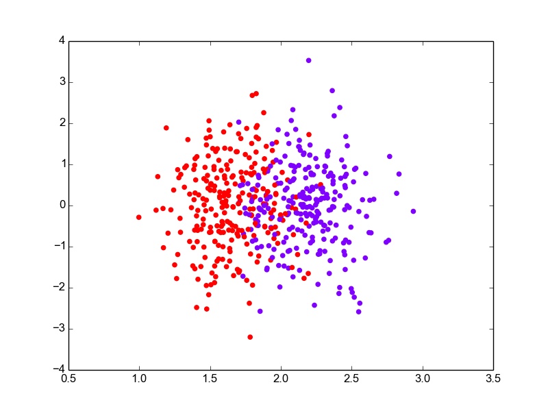
-
Digits is a dataset of handwritten digits 0 - 9. It has 64 dimensional data with 10 classes. I used this data as it was for classification. For this dataset, I perform the projection of data into 2 dimensions and then use bivariate Gaussian modeling for classification. After evaluation, the error rate comes out to be ~30% on the test set, which is not bad considering the 64-dimesional, 10-class data is projected to 2-D. For the 2-dimensional scatter plot for the data projections looks like this.
LDA : 2-D Projections for Digits data 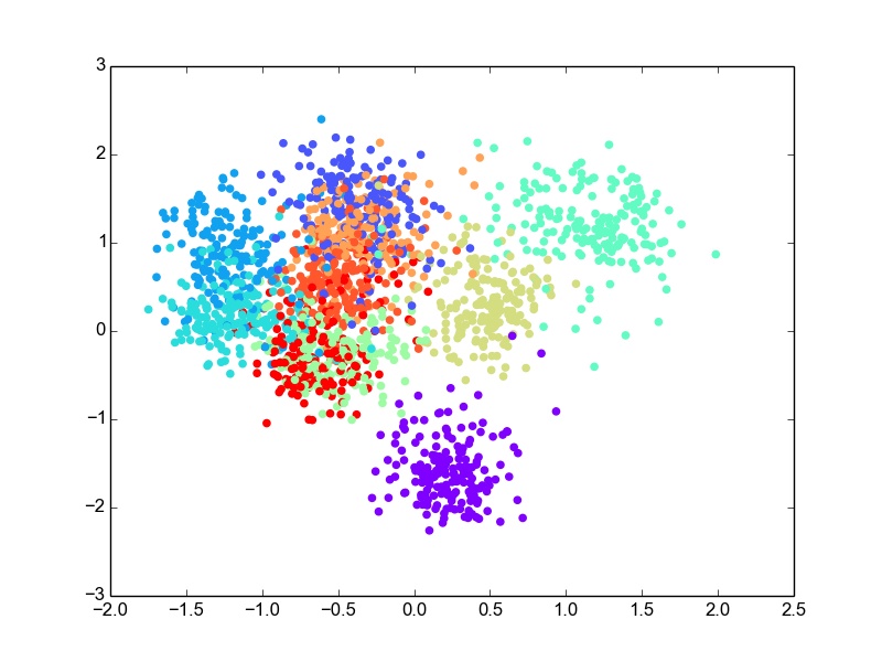
Though there is overlap in the data in 2-D, some classes are well separated as well. The overlap is expected due to the very-low dimensional projection. I think given this constraint, LDA does a good job at projection. I thought it would be fun to plot the likelihood gaussian curves as well. So here is the code to do that and the plot obtained.
def plot_bivariate_gaussians(self):
    classes = list(self.means.keys())
    colors = cm.rainbow(np.linspace(0, 1, len(classes)))
    plotlabels = {classes[c] : colors[c] for c in range(len(classes))}

    fig = plt.figure()
    ax3D = fig.add_subplot(111, projection='3d')
    for c in self.means.keys():
        data = np.random.multivariate_normal(self.gaussian_means[c],
                                             self.gaussian_cov[c], size=100)
        pdf = np.zeros(data.shape[0])
        cons = 1./((2*np.pi)**(data.shape[1]/2.)*np.linalg.det(self.gaussian_cov[c])**(-0.5))
        X, Y = np.meshgrid(data.T[0], data.T[1])
        def pdf(point):
            return cons*np.exp(-np.dot(np.dot((point-self.gaussian_means[c]),np.linalg.inv(self.gaussian_cov[c])),(point-self.gaussian_means[c]).T)/2.)

        zs = np.array([pdf(np.array(ponit)) for ponit in zip(np.ravel(X),
                                                               np.ravel(Y))])
        Z = zs.reshape(X.shape)
        surf = ax3D.plot_surface(X, Y, Z, rstride=1, cstride=1,
                                   color=plotlabels[c], linewidth=0,
                                   antialiased=False)
    plt.show()
LDA : Projected data likelihood Gaussian plots for Digits data 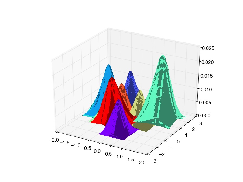
- Bishop, C. M. (2006). Pattern recognition. Machine Learning, 128.
I used two datasets - Boston housing data and the Digits data.